Kernel Methods
Kernel methods aim to quantify dissimilarity between microbial communities. By defining a distance between two microbial communities, it is possible to perform classification and cluster communities obtain a high level understanding of how microbial communities are impacted by specific environmental variables.
One of the most commonly used distance metrics used in microbial ecology is Unifrac. Unifrac incorporates information from prior knowledge of the evolutionary history of the microbes, in addition to the observed microbial abundances.
To illustrate how Unifrac works, consider the following example
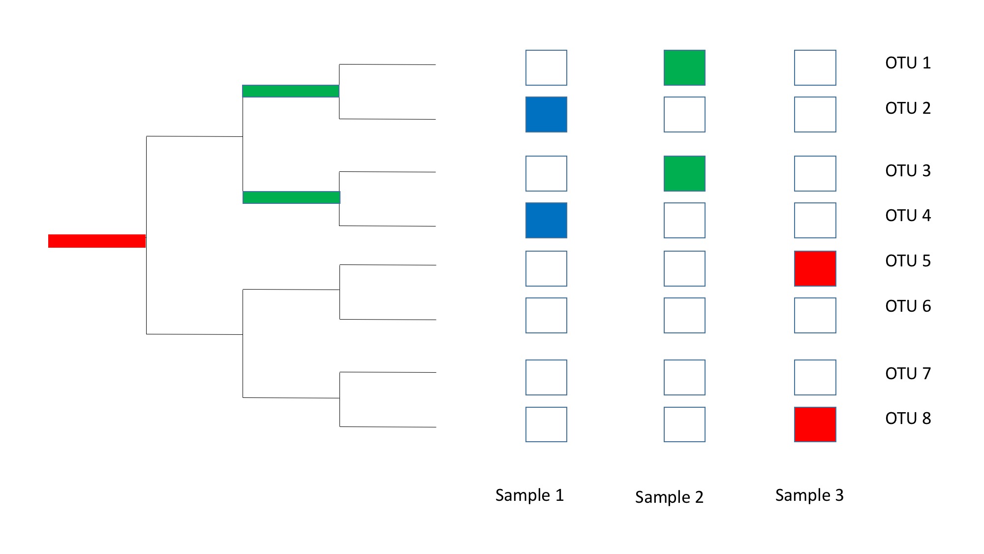
Here, there are three samples that contain microbial communities made up 9 different species. None of the communities have any species in common, but we can see that the species between Sample 1 and Sample 2 are more similar compared to the species between Sample 1 and Sample 3. This is because the species between Sample 1 and Sample 2 share a common ancestor that is more recent than Sample 3.
This is how Unifrac attempts to resolve the differences between microbial communities. To account the underlying phylogeny, Unifrac will calculate the differences between the common ancestor abundances between the samples. In fact, Unifrac has been shown to be a variant of the Earth Mover's Distance and can be thought of as a technique that calculates the flow of species abundances through the common ancestors between microbial communities.
To show how to run Unifrac, let's first create the familar RNA copy number simulation shown in the PVA tutorial. We'll first want to boot up rpy2 to embed R inside of Python. We want to do this, since we will be using the scikit-bio implementation of Weighted Unifrac.
import warnings
warnings.filterwarnings("ignore")
%load_ext rpy2.ipython
%%R -o OTUTable -o disturbance_frequency

library(ape)
library(phytools)
library(magrittr)
library(nlme)
set.seed(1)
tree <- rtree(10)
n <- 25
disturbance_frequency <- rexp(n) %>% sort %>% log

Q <- diag(9) %>% cbind(rep(0,9),.) %>% rbind(.,rep(0,10))
Q <- Q+t(Q)-diag(10)
# Q <- Q
RNAcopyNumber <- sim.history(tree, Q, anc = '3')


abundances <- function(dst,RNAcopy){
  m <- length(RNAcopy)
  muTot <- 1e4   ##a mean of 10,000 sequence counts per sample.
  logmu <- 3 * dst * log(RNAcopy) #model to yield linear changes in log-ratios
  muRel <- exp(logmu) / sum(exp(logmu))  #mean relative abundances
  mu = muRel * muTot
  size = 1
  N <- rnbinom(m, size, mu=mu)
}

OTUTable <- sapply(as.list(disturbance_frequency),
                   FUN=function(dst, c) abundances(dst, c),
                   c=as.numeric(RNAcopyNumber$states)) %>% matrix(., ncol=n, byrow=F)
OTUTable <- as.data.frame(OTUTable)
rownames(OTUTable) <- names(RNAcopyNumber$states)
write.tree(tree, file='tree.nwk', tree.name=TRUE)
Now we'll want to read in the tree and table from simulation. Once the data is formated correctly, we can run Weighted Unifrac to obtain a pairwise distance matrix. This distance matrix will enumerate the distances of all possible pairs of samples.
from skbio import TreeNode
from skbio.diversity import beta_diversity
tree = TreeNode.read('tree.nwk')
table = OTUTable.astype(int).T
wu_dm = beta_diversity("weighted_unifrac", table.values, table.index, tree=tree,
                        otu_ids=table.columns)
We can plot the distance matrix to see which samples are most similar to each other using Unifrac.
wu_dm
From here, we can see that samples V1 through V10 have small distances, suggesting that these communities are similar to each other. This makes since, because these communities are primarily composed of low RNA copy number microbes. Whereas the samples V1 through V10 are very different to V15 through V25. This is also expected, since V15 through V25 are composed of high RNA copy number species, and are very phylogenetically dissimilar due to our simulation.
To show that incorporating the phylogeny is useful, let's run Bray Curtis to see how well that can differentiate these samples.
bc_dm = beta_diversity("braycurtis", table.values, table.index)
bc_dm
As we can see here, Bray Curtis is able to highlight the differences between the V1-V10 and V15-V25 communities. However, because this metric is agnostic to underlying phylogeny, it mistakenly identifies the low RNA copy number communities to be dissimilar communities.
To obtain a high level understanding of how these sample differ, it is common to use Principal Coordinates Analysis to embed these samples into a scatter. These plots can help provide intuition about which environmental factors are driving the separation between communities. We will use this technique with the Unifrac distances. to see if Disturbance Frequency is the variable that explains this difference.
import pandas as pd
from skbio.stats.ordination import pcoa

samp_md = pd.DataFrame(disturbance_frequency, index=table.index, columns=['Disturbance_Frequency'])
pc = pcoa(wu_dm)
pc.plot(samp_md, 'Disturbance_Frequency',
        axis_labels=('PC 1', 'PC 2', 'PC 3'),
        title='Disturbance_Frequency', cmap='jet', s=50)

As expected, the disturbance frequency appears to be the primary factor explaining separation between the microbial communities.
Summary - Kernel Methods
In conclusion, Kernal Methods are very useful tools for obtaining a high level understanding about which environmental variables explain the differences between microbial communities. Methods that can incorporate phylogeny such as Unifrac are key for recovering patterns with phylogenetically relevant information. We've seen here that failing to incorporate phylogeny could lead to misleading interpretation about the underlying system.